As credit risk became an increasing concern in recent years, various advanced methods have been employed extensively to measure credit risk exposures. Nowadays, structural and reduced form models represent the two primary classes of credit risk modeling approaches. The structural approach aims to provide an explicit relationship between default risk and capital structure, while the reduced form approach models credit defaults as exogenous events driven by a stochastic process (such as a Poisson jump process).

Under structural models, a default event is deemed to occur for a firm when its assets reach a sufficiently low level compared to its liabilities. These models require strong assumptions on the dynamics of the firm’s asset, its debt and how its capital is structured. Merton model was the first structural model and has served as the cornerstone for all other structural models. To illustrate key concepts behind structural approach, we will review Merton model in detail, and briefly introduce some important extensions to this model.

The Merton Model (1974)

The real beauty of Merton model lies in the intuition of treating a company’s equity as a call option on its assets, thus allowing for applications of Black-Scholes option pricing methods. This analogy is justified by the concept of a limited liability company. The shareholder of such a company puts in a certain amount of equity, with which the company incurs debt to carry its business. Suppose at time t the company has asset \(A_t\) financed by equity \(E_t\) and zero-coupon debt \(E_t\) of face amount \(K\) maturing at time \(T\) satisfying the balance sheet relationship

As the company trades, its assets may either appreciate or depreciate in value. If the assets appreciate in value such that \(A_T > K\), the debt holders do not get to share the profits – they are entitled to no more than repayment of the debt, which is \(K\) and shareholders pick up all the appreciation in the value of assets, which is \( A_T - K \). However, if the assets decline to a value that cannot cover the amount repayable on debt (\(A_T \leq K\)), in which case debt holders have the first claim on residual asset \(A_T\) and shareholders are left with nothing (and the firm goes bankrupt). Therefore, equity value at time \(T\) can be written as:

and so equity can be viewed as a European call option on the firm’s assets. It follows that the well-known option pricing formulas can be applied if some modeling assumptions are made. Let us assume that the asset value \(A_t\) of a firm follows a geometric Brownian motion process, with dynamics under the real-world measure \(P\) given by

where \(\mu\) is the mean rate of return on the assets and \(\sigma\) is the asset volatility. Under risk-neutral settings this becomes

where \(r\) is the risk-free rate. Further assumptions are needed for this model to work, such as there are no bankruptcy charges, meaning the firm’s liquidation value equals its book value; the debt and equity are frictionless tradeable assets i.e. incurring no transaction costs.

The equity value at time \(t < T\) can be found using the familiar Black-Scholes call option formula

where \(N(.)\) denotes the standard normal cumulative distribution function, and

Under this framework, a credit default at time T is triggered by the event that shareholders’ call option matures out-of-money, with a risk-neutral probability

which can be converted into a real-world probability by switching to measure \(P\), which gives

where \(d_2^P = \frac{\log (A_t/K)+(\mu - \sigma^2/2)(T-t)}{\sigma\sqrt{T-t}}.\)

Debt holders, on the other hand, receive

Thus debt holders, lest they should be exposed to default risk, can hedge their position by purchasing a European put option written on the same underlying asset \(A_t\) with strike price \(K\), whose payoff is exactly \((K- A_T)^+\). Combining these two positions (debt and put option) would guarantee a payoff of \(K\) for debt holders at time \(T\), thus forming a risk-free position

where \(P_t\) is the price of the put option at time \(t\), which can be determined by applying the Black-Scholes formula for put option

The corporate debt is a risky bond, and thus should be valued at a credit spread (risk premium). Let \(s\) denote the continuously compounded credit spread – the difference between the (promised) yield on the risky bond and the yield on a riskless bond – then bond price \(D_t\) can be written as

Thus we can solve for \(s\)

which allows us to compute credit spread when \(A_t\) and \(\sigma\) are available for given \(t, T, K\), and \(r\).

Term structure of credit spread under Merton Model

The term structure of credit spread refers to a plot of spreads against maturities. By varying \(T\), we obtain the term structure of credit spreads implied by the Merton model, which according the above formula depends on the following variables

• the volatitlity of firm’s total value \(\sigma\),
• the risk-free rate \(r\),
• the face value of debt \(K\),
• the current value of the firm \(A_t\), and
• the time to maturity \(T- t\)

Below is an R function that help us compute the credit spread for specified input variables

# Function to compute credit spread in a Merton model
# Input variables:
## A : current firm value
## K : face value of zero-coupon debt
## tau : time to maturity
## sigma : volatility of firm value
## r : risk-free rate

spreadMerton <- function(A, K, tau, sigma, r){
d1 <- (log(A/K)+(r+sigma^2/2)*tau)/(sigma*sqrt(tau))
d2 <- d1 - sigma*sqrt(tau)
s <-  -1/tau*log(pnorm(d2)+A*exp(r*tau)*pnorm(-d1)/K)
return (s)
}

To obtain the term structure, we let the time to maturity vary from 1 to 10 years while keeping the other variables fixed. In particular, \(A_t = 100, K = 60, \sigma = 0.3\), and \(r = 0.1\). The term structure is plotted below.

A <- 100
K <- 60
tau <- 1:10
sigma <- 0.3
r <- 0.1

library("ggplot2")

spread <- spreadMerton(A, K, tau, sigma, r)*1e4
df <- as.data.frame(cbind(tau, spread))
plot1 = ggplot(df, aes(x = tau, y = spread)) + geom_point() + geom_line(aes(y=spread)) + labs(x="Maturity (yrs)", y="Spread (bps)")
plot1 + theme(panel.grid.major = element_blank(), panel.grid.minor = element_blank())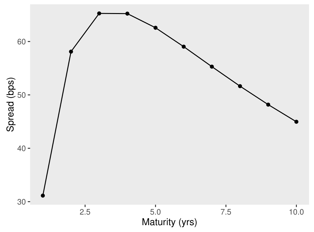

Notice the humped shape of the plot. Spreads are low at short maturities, increase with maturity initially, and then decline at longer maturities. This shape is typical of what obtains in the Merton model when \(A_t > K\). Intuitively, for very short maturities, default is an unlikely event, so spreads are low. As maturity lengthens, there is sufficient time for the bond to default as the firm value may drop below the value of debt, thereby resulting in higher spreads. For much longer maturities, the spread declines because, conditional on the bond not having defaulted for some time, the likelihood of the firm being far from default is high on average, thereby resulting in a lower probability of default. In what follows, we will consider how the debt level (leverage) can affect the shape of the term structure of credit spreads.

The Impact of Leverage

We measure leverage by the ratio of the face value of debt \(K\) to the initial (time \(t\)) value of the firm \(V_t\). The figure below presents the spread curves for three different values of leverage: 50%, 65%, and 80%. The volatility of firm value is taken to be 25%, and the risk-free rate is 5%. The spreads are reported in basis points.

library("reshape2")

tau <- seq(1,10,by=0.25)
low <- spreadMerton(100,50,tau,0.25,0.05)*1e4
medium  <- spreadMerton(100,65,tau,0.25,0.05)*1e4
high <- spreadMerton(100,80,tau,0.25,0.05)*1e4
df <- as.data.frame(cbind(tau, low, medium, high))
colnames(df)[-1] <- c("Low Leverage", "Medium Leverage", "High Leverage")
df_long <- melt(df, id="tau")
colnames(df_long)[2] <- c("Debt")
plot1 = ggplot(data=df_long, aes(x=tau, y=value, colour=Debt)) + 
geom_line() + geom_point() + labs(x="Maturity (yrs)", y="Spread (bps)")
plot1 + theme(panel.grid.major = element_blank(), panel.grid.minor = element_blank(), legend.position="bottom")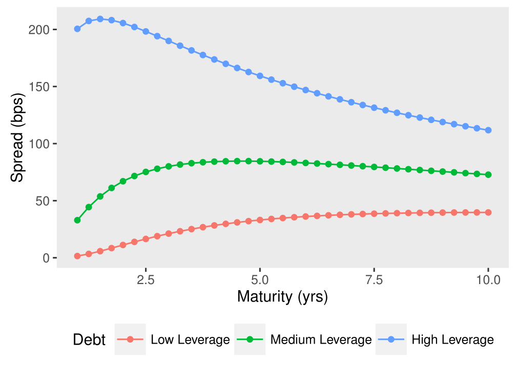

We observe the followings:

• A low-leverage company has a flatter credit spread term structure with initial spreads close to zero since it has sufficient assets to cover short-term liabilities. Spread slowly increases with debt maturity (reflecting future uncertainties), before it starts to decrease at the long end.
• A medium-leverage company has a humped-shape credit spread term structure. The very short-term spreads are low as the company currently has just enough assets to cover debts. Spread then rises quickly since asset value fluctuations could easily result in insufficient assets, before it gradually drops for longer maturities.
• A high-leverage company has a downward-sloping credit spread term structure which starts very high and decreases for longer maturities as more time is allowed for the company’s assets to grow higher and cover liabilities.

Thus it appears the credit spread curve implied by Merton model is realistic after all. However, empirical studies have shown that Merton model tends to underestimate credit spreads, particularly short-term spreads. This is due to the technical assumptions of the asset value following a Brownian motion, which evolves continuously. So if \(A_t > K\) then it is unlikely over short horizons that the value will drop below \(K\) and trigger a default. Another limitation of Merton model is that it assumes a default can only happen at maturity, meaning regardless of what the intermediate values of \(A_t\) are, as long as \(A_T > K\) then the possibility of a default at all is precluded. Nevertheless, the Merton model is still a great starting point for studying credit risk, and continues to serve as a premise for other models to extend upon.

References

1. Yu Wang.”Structural Credit Risk Modeling: Merton and Beyond”. In: Risk Management 16 (2009).
2. Lecture notes. https://www.fields.utoronto.ca/programs/scientific/09-10/finance/courses/hurdnotes2.pdf.