Background
Using devices such as Jawbone Up, Nike FuelBand, and Fitbit it is now possible to collect a large amount of data about personal activity relatively inexpensively. These type of devices are part of the quantified self movement – a group of enthusiasts who take measurements about themselves regularly to improve their health, to find patterns in their behavior, or because they are tech geeks. One thing that people regularly do is quantify how much of a particular activity they do, but they rarely quantify how well they do it. In this project, your goal will be to use data from accelerometers on the belt, forearm, arm, and dumbell of 6 participants. They were asked to perform barbell lifts correctly and incorrectly in 5 different ways. More information is available from the website here: http://groupware.les.inf.puc-rio.br/har (see the section on the Weight Lifting Exercise Dataset).
Data description
The training data for this project are available here:
https://d396qusza40orc.cloudfront.net/predmachlearn/pml-training.csv
The test data are available here:
https://d396qusza40orc.cloudfront.net/predmachlearn/pml-testing.csv
The data for this project come from this source: http://groupware.les.inf.puc-rio.br/har. [1]
Objectives
The goal of your project is to predict the manner in which they did the exercise. This is the classe variable in the training set.
Two models will be tested using decision tree and random forest algorithms. The model with the highest accuracy and lowest out-of-sample error will be chosen as our final model.
Libraries
library(caret)
library(rpart)
library(rpart.plot)
library(randomForest)
library(rattle)
Getting and cleaning training data
Some missing values are coded as string “#DIV/0!”, “”, or “NA” – we will change them all to “NA” for consistency. We then remove variables that are irrelevant to our prediction, namely user_name, raw_timestamp_part_1, raw_timestamp_part_2, cvtd_timestamp, new_window, and num_window (columns 1-7), and also exclude those with more than 95% missing values.
urlTrain <- "http://d396qusza40orc.cloudfront.net/predmachlearn/pml-training.csv"
urlTest <- "http://d396qusza40orc.cloudfront.net/predmachlearn/pml-testing.csv"
train <- "pml-training.csv"
test <-  "pml-testing.csv"

#Original training data set
if (file.exists(train)) {
  train <- read.csv(train, na.strings=c("#DIV/0!","","NA"))
} else {
  download.file(urlTrain,train)
  train <- read.csv(train, na.strings=c("#DIV/0!","","NA"))
}

train <- train[,-c(1:7)]

NArate <- apply(train, 2, function(x) sum(is.na(x)))/nrow(train)
train <- train[!(NArate>0.95)]
dim(train)
## [1] 19622 53
#Original testing data set
if (file.exists(test)) {
  test <- read.csv(test, na.strings=c("#DIV/0!","","NA"))
} else {
  download.file(urlTest,test)
  test <- read.csv(test, na.strings=c("#DIV/0!","","NA"))
}
test <- test[,-c(1:7)]
NArate <- apply(test, 2, function(x) sum(is.na(x)))/nrow(test)
test <- test[!(NArate>0.95)]
dim(test)
## [1] 20 53
After cleaning, the training data set contains 53 variables and 19622 observations, and the testing data set has 53 variables and 20 observations. These are the variables that will be used for prediction.
Cross-validation
Cross-validation will be performed by subsampling our training data set randomly without replacement into 2 subsamples: subTrain data (70% of the original training data set) and subTest data (remaining 30%).
set.seed(16)
training <- createDataPartition(y=train$classe,p=.70,list=F)
subTrain <- train[training,]
subTest <- train[-training,]
Prediction using Decision Tree
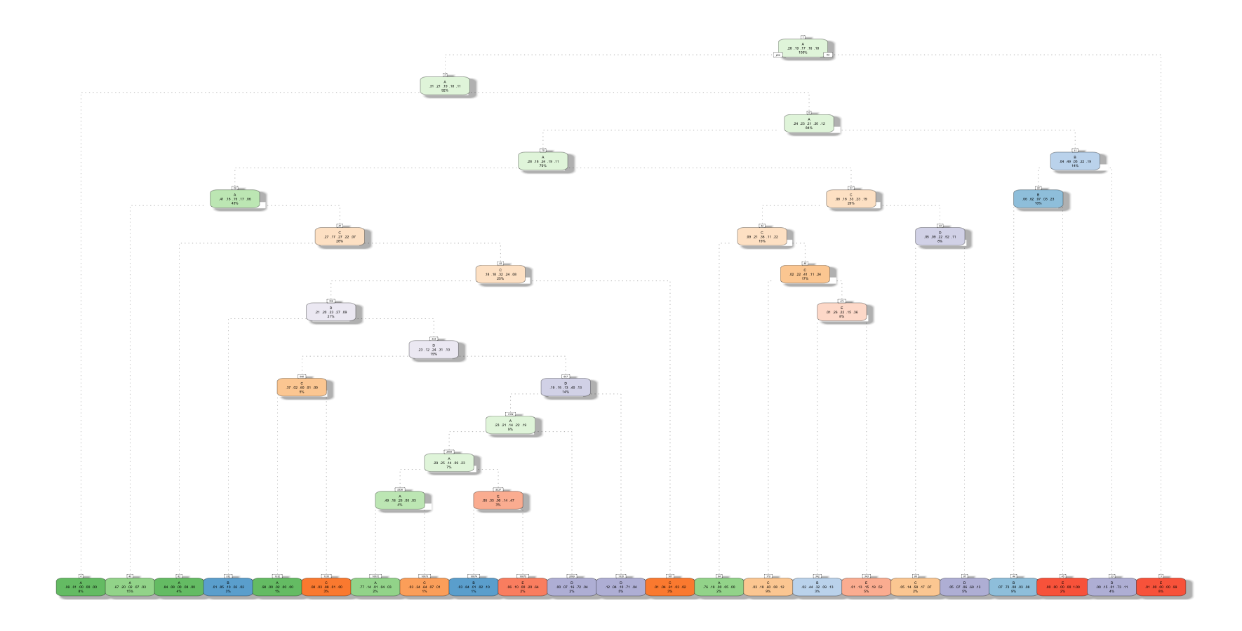
model1 <- rpart(classe ~ ., data=subTrain, method="class")
predict1 <- predict(model1, subTest, type = "class")
fancyRpartPlot(model1)
confusionMatrix(predict1, subTest$classe)
## Confusion Matrix and Statistics
##
##           Reference
## Prediction    A    B    C    D    E
##          A 1498  239   24   85   30
##          B   52  635  124   50   99
##          C   39  132  773   98   75
##          D   68   70   77  635   83
##          E   17   63   28   96  795
##
## Overall Statistics
##
##                Accuracy : 0.7368
##                  95% CI : (0.7253, 0.748)
##     No Information Rate : 0.2845
##     P-Value [Acc > NIR] : < 2.2e-16
##
##                   Kappa : 0.6658
##  Mcnemar's Test P-Value : < 2.2e-16
##
## Statistics by Class:
##
##                      Class: A Class: B Class: C Class: D Class: E
## Sensitivity            0.8949   0.5575   0.7534   0.6587   0.7348
## Specificity            0.9102   0.9315   0.9292   0.9394   0.9575
## Pos Pred Value         0.7985   0.6615   0.6920   0.6806   0.7958
## Neg Pred Value         0.9561   0.8977   0.9469   0.9336   0.9413
## Prevalence             0.2845   0.1935   0.1743   0.1638   0.1839
## Detection Rate         0.2545   0.1079   0.1314   0.1079   0.1351
## Detection Prevalence   0.3188   0.1631   0.1898   0.1585   0.1698
## Balanced Accuracy      0.9025   0.7445   0.8413   0.7991   0.8461
We can see that the accuracy is 73.68%. Let’s try using Random Forests to see if we can get a better accuracy.
Prediction using Random Forest
model2 <- randomForest(classe ~. , data=subTrain)
predict2 <- predict(model2, subTest, type = "class")
confusionMatrix(predict2, subTest$classe)
## Confusion Matrix and Statistics
##
##           Reference
## Prediction    A    B    C    D    E
##          A 1672    5    0    0    0
##          B    2 1134    3    0    0
##          C    0    0 1022    8    1
##          D    0    0    1  956    2
##          E    0    0    0    0 1079
##
## Overall Statistics
##
##                Accuracy : 0.9963
##                  95% CI : (0.9943, 0.9977)
##     No Information Rate : 0.2845
##     P-Value [Acc > NIR] : < 2.2e-16
##
##                   Kappa : 0.9953
##  Mcnemar's Test P-Value : NA
##
## Statistics by Class:
##
##                      Class: A Class: B Class: C Class: D Class: E
## Sensitivity            0.9988   0.9956   0.9961   0.9917   0.9972
## Specificity            0.9988   0.9989   0.9981   0.9994   1.0000
## Pos Pred Value         0.9970   0.9956   0.9913   0.9969   1.0000
## Neg Pred Value         0.9995   0.9989   0.9992   0.9984   0.9994
## Prevalence             0.2845   0.1935   0.1743   0.1638   0.1839
## Detection Rate         0.2841   0.1927   0.1737   0.1624   0.1833
## Detection Prevalence   0.2850   0.1935   0.1752   0.1630   0.1833
## Balanced Accuracy      0.9988   0.9973   0.9971   0.9955   0.9986
As expected, random forest algorithm performed better than Decision Trees, producing an accuracy level of 99.6%. Hence the random forest-based prediction model is chosen.
Discussion
In this project, 19622 observations recorded from 6 individuals performing weight lifting exercises were used to analyze and predict how well (or badly) an activity is performed given a different set of observations. 70% of the total observations were used to build a model by random forest algorithm, and the remaining 30% of the observations were used for cross-validation. The model statistics showed that the built model had the overall accuracy of over 99% for the testing set, which is not overlapping with observations used to built the model. Overall, the model is well developed for prediction.
Accuracy is the proportion of correct classified observation over the total sample in the subTest data set. Expected accuracy is the expected accuracy in the out-of-sample data set (i.e. original testing data set). Thus, the expected value of the out-of-sample error will correspond to the expected number of missclassified observations divided by total observations in the test data set, which is (1-accuracy) in the cross-validation data (subTrain and subTest).
References
[1] Velloso, E.; Bulling, A.; Gellersen, H.; Ugulino, W.; Fuks, H. Qualitative Activity Recognition of Weight Lifting Exercises. Proceedings of 4th International Conference in Cooperation with SIGCHI (Augmented Human ‘13) . Stuttgart, Germany: ACM SIGCHI, 2013.