The binomial tree model (BTM) is an intuitive lattice-based method that is frequently used in derivative pricing, particularly American-style derivatives. They are also flexible since only nominal changes of the payoff function are needed for dealing with complex, nonstandard option payoff function.
The basic building block of BTM is the one-step binomial model where an asset today can either go up or go down in value at a future time, which might, for example, be tomorrow, or next month, or next year. In this simple situation “risk neutral pricing” can be defined and the model can be applied to price forward contracts, exchange rate contracts and interest rate derivatives. By considering more than one-step a full binomial tree can be constructed, where the price that an asset has branches out, either upward or downward at each point in time. When the number of steps, or periods, is reasonably large these binomial trees can provide a remarkable good approximation to a more complex stochastic process in a continuous time setting.

Delta Hedging

Buying a stock is a risky investment. Buying a call option whose value is contingent on that stock is even more so. Yet combining said stock and option can produce an investment that risk-free. That means it is possible to hedge a position in a stock by taking an opposite position in the option. To create such a risk-free investment we have to create a portfolio with both the stock and option in exactly the right proportions so that their risks eliminate each other. The number of units of the stock required per option is known as the \(\Delta\) (Delta) of the stock and taking these positions to create a risk-free investment is known as Delta Hedging.

But how do we calculate such a \(\Delta\)? Consider the following example.

The underlying stock is currently priced at 100 and at the end of three months it has either risen to 175 or has fallen to 75. A call option on this stock is at the money with a strike price of 100.

There is an “up” state and a “down” state. Let \(u = 0.75\) and \(d = -0.25\), so that the value of the stock in three months in the up state is \(100(1+u) = 175\) and the value in the down state is \(100(1 + d) = 75\), which is not risk-free. If the stock goes up then in 3 months the call can be exercised for a payoff of \(175 - 100 = 75\) and if the price of the stock goes down, then the call will expire worthless (unexercised). Thus the payoff of the call option is 75 in the up state and 0 in the down state, which is not risk-free, either. Suppose however, that we consider buying \(\Delta\) units of the stock and writing (shorting) one call. The payoff from this portfolio is \(175 \Delta - 75\) in the up state – because the stock has now gone up to 175 but the call option will be exercised against us, hence our obligation of 75. The payoff in the downstate is simply \(75\Delta\) as the call option is not exercised. To make this portfolio risk-free it’s necessary to choose \(\Delta\) such that

\[175 \Delta - 75 = 75 \Delta\]

so that the payoff is the same no matter whether we are in the up state or the down state. Solving for \(\Delta\) we get \(\Delta = 3/4\), which means for every 3 shares of stock we buy, we should sell 4 call options to fully hedge our position and make our portfolio worth \(75 \times 3/4 = 56.25\) at the end of 3 months, however the underlying stock moves. Assuming there are no arbitrage opportunities the portfolio can be valued using risk-free rate.

Now suppose the risk-free rate is given by \(r = 0.1\) (annualized), then the present value of our portfolio is \(56.25 / (1+0.1/4) = 54.878\). The value of the portfolio now is simply the current value of the current value of the shares, \(3/4 \times 100 = 75\) less \(c\), the price of one call option. Therefore

\[75 - c = 54.878.\]

This gives \(c = 20.122\).

What if the given risk-free rate is continuously compounded? In that case we only need to change the present value of our portfolio to \(56.25e^{-0.1/4} = 54.861\) and recalculate \(c\).

Risk neutral pricing

The same procedure can be generalized. Let \(S_0\) be the current value of the underlying stock, so its terminal value is either \(S_0u\) in the up state or \(S_0d\) in the down state.

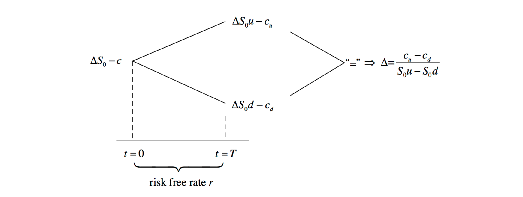
If the risk-free rate is continuously compounded, the price of the option can be found by

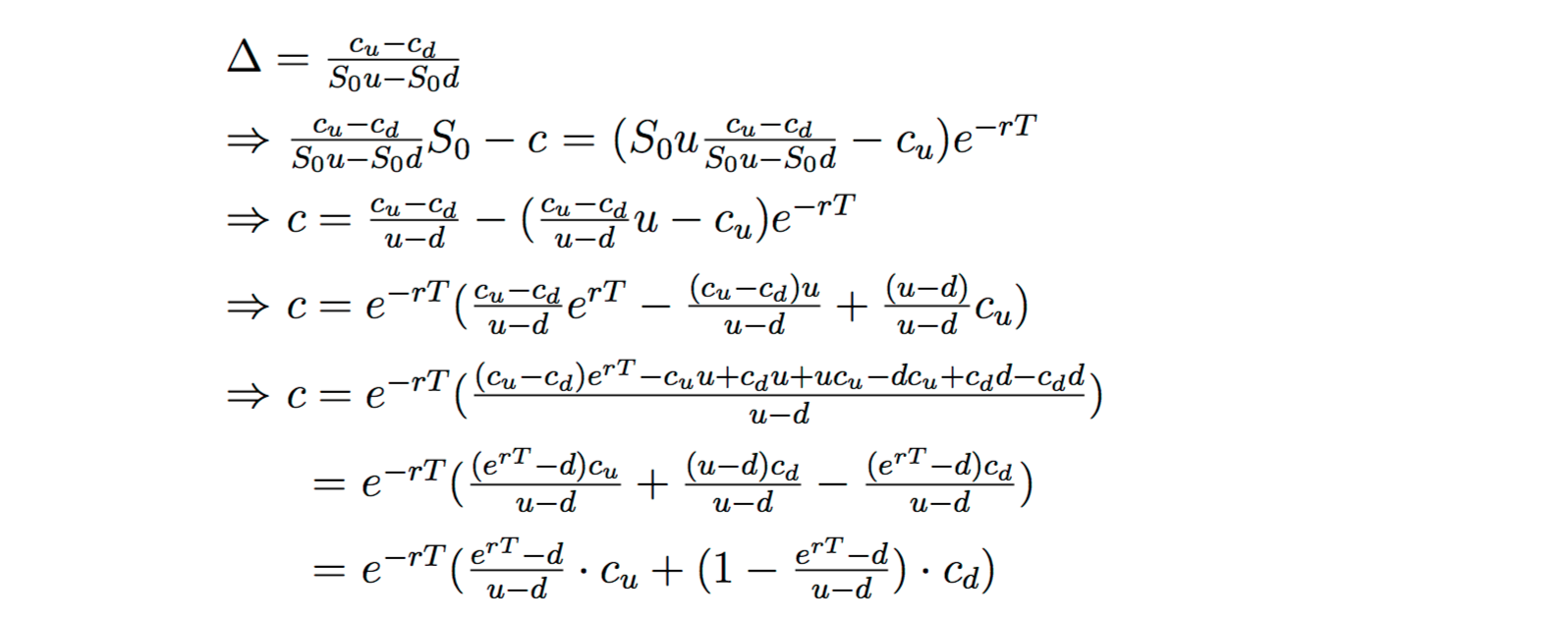
or \(c = e^{-rT}(pc_u + (1-p)c_d)\) where \(p = \frac{e^{rT}-d}{u-d}\).

Similarly if \(r\) is discretely compounded, then

\[c = (1+rT)^{-1}(pc_u + (1-p)c_d)\]

where \(p = \frac{1+rT-d}{u-d}\)

The above expressions for \(c\) are known as risk-neutral pricing formulas and \(p\) risk-neutral probabilities.

Multi-period Binomial Tree Model

We now move from the one-period model to a multi-period model. Previously we assumed that, given an initial price of \(S_0\), the price of a stock could increase by a factor of \(u\) or decrease by a factor of \(d\) after the first period. Now assume that after the second period, the stock price can again increase or decrease by the multiplicative factors u and d, respectively. Then at the end of the second period, the possible stock prices are \(u^2 S_0\), \(udS_0 = duS_0\), and \(d^2S_0\). Continuing this pattern for multiple time steps give a full binomial tree of possible stock prices.

References

1. John van der Hoek and Robert J. Elliott. “Binomial Models in Finance”. Springer (2006).