Problem Statement

The environment is called LunarLander-v2 which is part of the Python gym package @lunarlander. An episode always begins with the lander module descending from the top of the screen. At each step, the agent is provided with the current state of the space vehicle which is an 8-dimensional vector of real values, indicating the horizontal and vertical positions, orientation, linear and angular velocities, state of each landing leg (left and right) and whether the lander has crashed. The agent then has to make one of four possible actions, namely do nothing, fire left orientation engine, fire main engine, or fire right orientation engine. These are 4 levers the agent must learn to control in order to land safely.

The scoring system is clearly laid out in OpenAI’s environment description. “Reward for moving from the top of the screen to landing pad and zero speed is about 100..140 points. If lander moves away from landing pad it loses reward back. Episode finishes if the lander crashes or comes to rest, receiving additional -100 or +100 points. Each leg ground contact is +10. Firing main engine is -0.3 points each frame. Solved is 200 points. Landing outside landing pad is possible, but is penalized. Fuel is infinite, so an agent can learn to fly and then land on its first attempt.”

The episode can also finish when it hits the maximum episode length of 1000 steps, as shown in the source code (max_episode_steps=1000). A successful solution is one that can get the agent consistently land on the target area safely i.e. with both legs touching the ground at (0, 0) at zero speed, yielding an average score of at least 200 points over 100 consecutive episode.

Exploratory Analysis

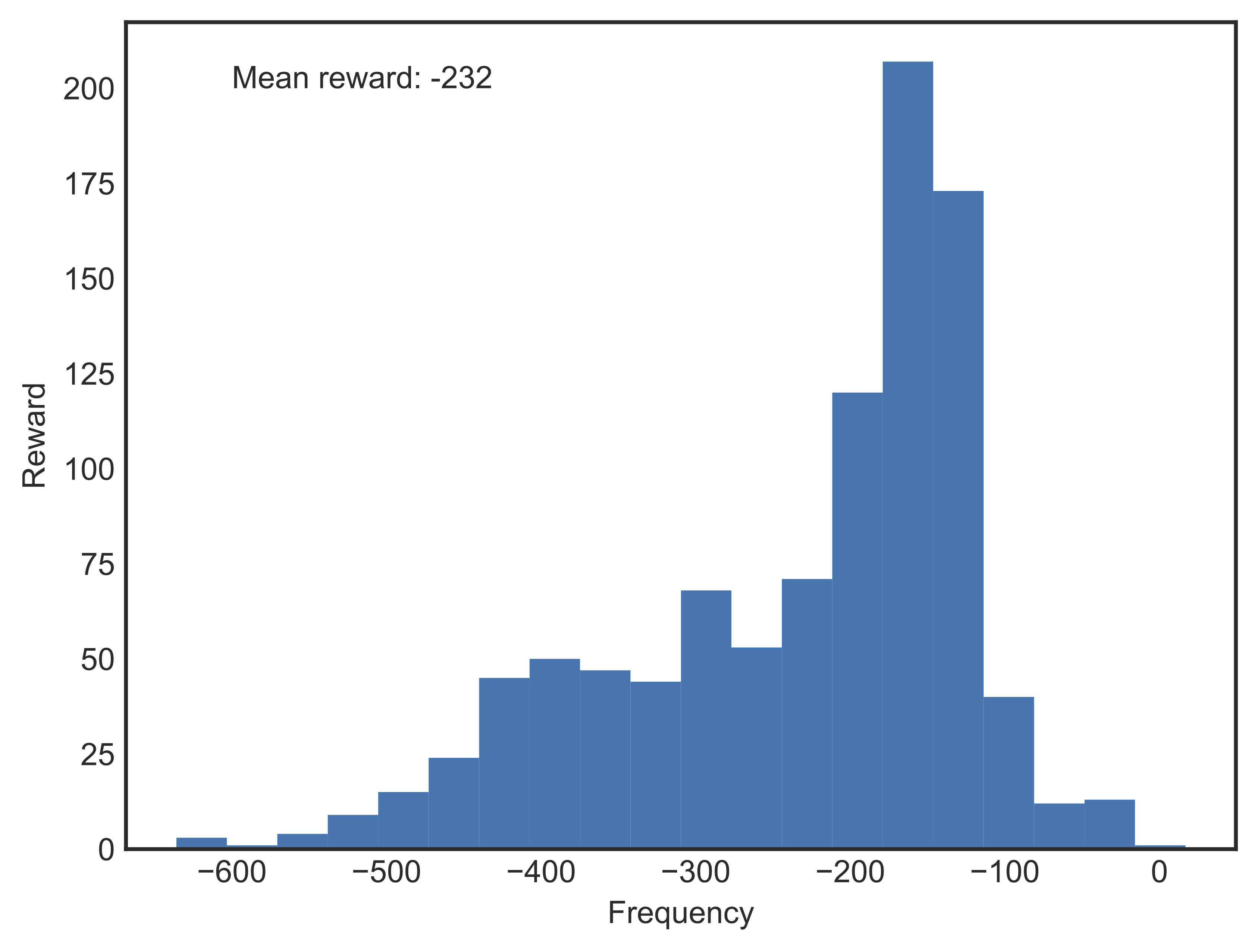
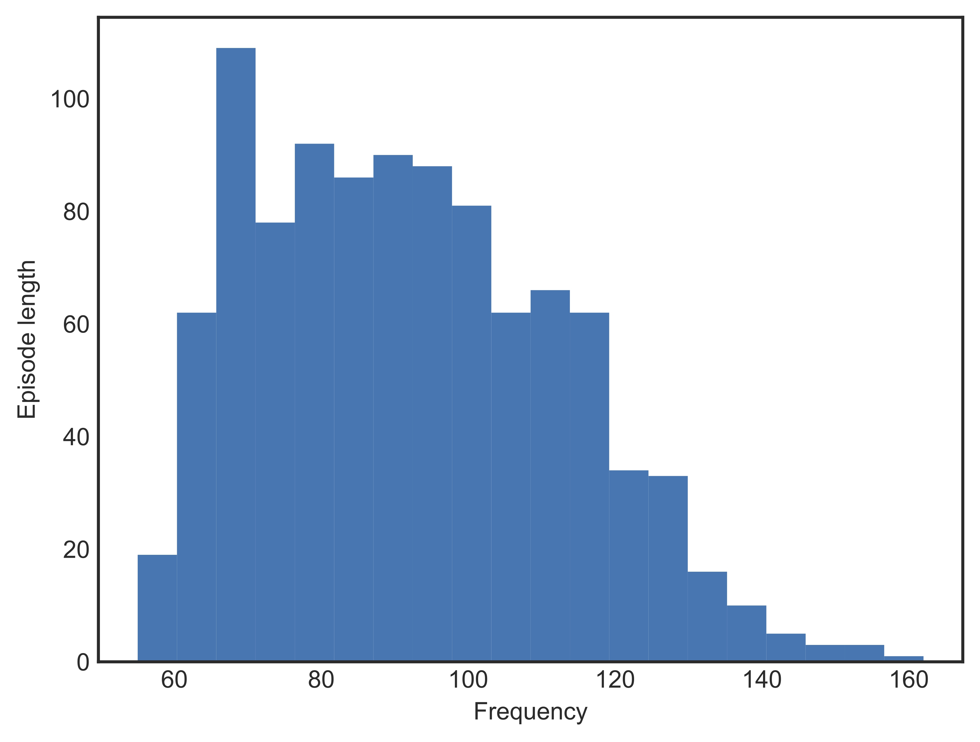
Without any assumptions or knowledge, the best way to explore is to randomly pick an action in each state and follow it. We ran 1000 episodes using a random agent, i.e. one that does not have any learning, to see if randomized exploration could help us win the game. Figures [fig:randagentreward] and [fig:randagentepslen] shows the performance of the random agent in terms of reward and episode length.

{width=”.35textwidth”}

{width=”.35textwidth”}

As expected, all episodes resulted in failure, with mean reward well below -200 indicating that the vehicle crashed most of the time. The chance of an unlearned agent landing is virtually nought. In addition, it didn’t take too long for an episode to finish; most episodes terminated in around 100 steps.

Techniques

Q-learning is one of the popular algorithms used in reinforcement learning because of its intuitiveness and simplicity. However it only works well with environments that have discrete state and action spaces. In addition, the space sizes must be relatively small, or else the Q-table would be too big and it would take ages to converge to the true Q-values. For our problem at hand, while the action space is discrete, the state space is continuous in 8 dimensions. Even though discretization of state space is possible, it is not a viable option since the memory requirement grows exponentially with number of discrete units chosen per state dimension. Interestingly, having a complex, continuous state space with a discrete set of actions is also characteristic of Atari games, which can be solved quite efficiently with a variant of deep Q-learning, called deep Q-network (DQN), proposed in @DBLP:journals/nature/MnihKSRVBGRFOPB15. This project employed a similar, albeit simpler, structure in which we omit the convolutional layers from the network.

DQN is simply an extension of a simple Q-network that is built upon tabular Q-learning. When the Q-table becomes too large to compute over as a result of infinitely many states, neural networks come to the rescue. By increasing the number of layers and nodes per layer, we can get a reasonably accurate function approximator that can map any number of possible states to their Q-values. While neural networks allow for greater flexibility, they come at a cost of stability: it turns out that Q-learning may suffer from instability and divergence when combined with an nonlinear Q-value function approximation and bootstrapping. DQN introduces two innovative additions that can stabilize training and allow for faster convergence:

• Experience replay: The reason why experience replay is helpful has to do with the fact that successive states are highly similar. This means that there is a significant risk that the network will completely forget about what it is like to be in state it has not seen in a while. This is detrimental to learning because catastrophic events that happened long ago might be forgotten and cannot be learned. Replaying experience prevents this by storing a fixed number of recent experiences (old ones will be discarded as new ones come in) in a memory replay buffer. From this buffer, we draw random batches of experiences, or “memories” to learn from and make updates to the network @dqnbeyond.

Experimental Details

Algorithm

{width=”.48textwidth”}

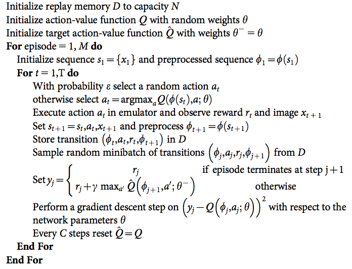
Our algorithm is largely similar to the one in Mnih et al, without the image processing parts. We also use Huber loss (called error clipping in @DBLP:journals/corr/MnihKSGAWR13) to avoid exploding gradients. For mean squared error loss (MSE) function, if the training sample does not align with current estimates, the gradient terms might explode and alter the network weights substantitally leading to undesirable performance. Huber loss function $H(e)= sqrt{1 + e^2}-1,$ where $e$ is the error between prediction and target value, has the advantage of being differentiable and has derivatives bounded between -1 and 1. Another deviation from the original paper is the use of $epsilon$-decay, which was implemented to exploit more optimal policies in later episodes.

Network Architecture

We omitted all convolutional layers as no processing of images is needed. The input to the network is a 8x1 tensor of real values indicating the current state of the lander, as described in [problemstatement]. The first fully-connected layer has 64 units, followed by another layer of 64 units, followed by another one of 32 units. All these layers are separated by Rectifier Linear Units (ReLU). Finally, the output layer is another fully-connected linear layer with a single output for each valid action. The optimization employed to train the network is Adam, with learning rate of 0.01. The size of the experience replay memory is 100,000 tuples. The memory gets sampled to update the network every 4 steps with minibatches of size 64.

Hyper-parameters

To find the best setting, we trained an agent for each combination of hyper-parameters for a maximum of 1000 episodes, regardless of the state of the agent. If an agent didn’t manage to accumulate a mean reward of 200 or greater for the last 100 training episodes within 1000 episodes, we said the agent did not complete learning. We then ran 10 independent trials, each consisting of 100 episodes, each episode having a maximum of 500 time steps, and took the average of the mean rewards of all 10 trials. Except for the three key hyper-parameters, namely discount rate ($gamma$), learning rate ($alpha$), and $epsilon$ decay, which we analyze in depth next, the rest of the hyper-parameters were held constant, including minibatch size, memory buffer capacity, and most importantly, the neural network architecture, the choice of optimizer, activation function, and loss function.

Discount rate

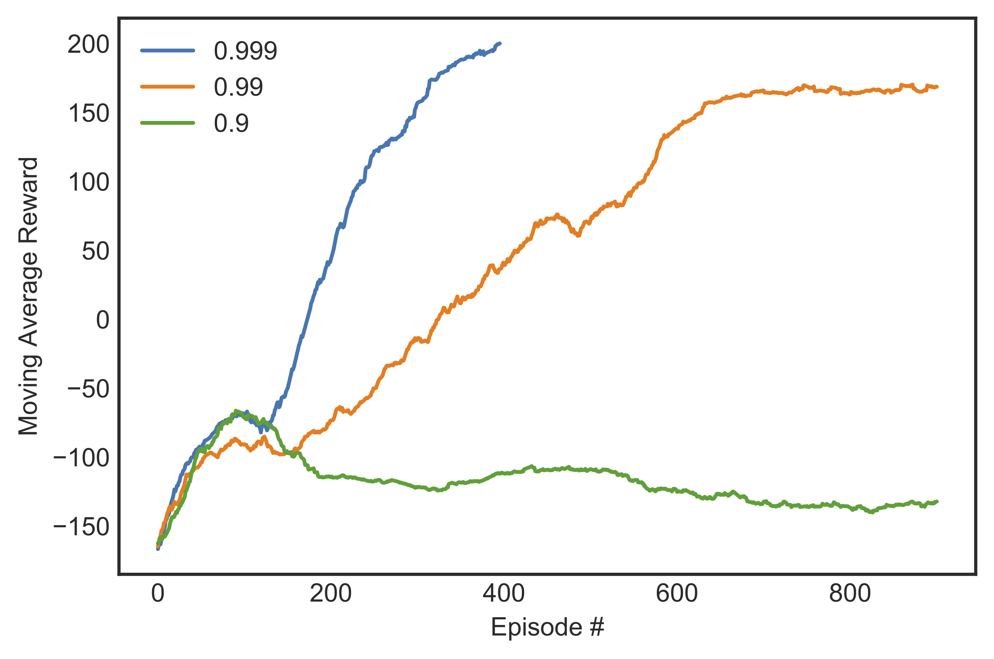
We considered a discount rate $gamma$ chosen from 0.9, 0.99, and 0.999. Figure [fig:marewardgamma] shows the learning curves for different discount rates with $epsilon$-decay $= 0.99$ and $alpha = 0.0005$.

{width=”.45textwidth”}

• $gamma=0.9$: The agent never completed learning, for all values of $alpha$ used. It crashed into the ground almost every time, and never managed a score of more than -100 in an episode. The reason is that with such a low $gamma$, the agent was only able to credit actions to success up to 10 steps into the future, which is too short a horizon.

• $gamma=0.99$: With a 100-step look-ahead ability, the agent could now land with varying degree of success. For small $alpha$ (0.001 or less), the agent landed without any crash very often, but seemed to be more concerned with landing than landing on target. Usually as soon as the vehicle’s legs touched the ground, all engines went off, regardless of whether it was at the landing pad or not. For bigger $alpha$’s, the agent did not complete learning.

• $gamma=0.999$: The agent now assigned credit up to 1,000 steps into the future, which is also the simulated environment’s limit. Similar to the case when $gamma=0.99$, the agent could only solve the problem with small learning rates and failed to do so if the learning rate gets bigger. However, when the agent could complete the training, it did so in fewer episodes than with $gamma=0.99$. The agent was now concerned with not only landing but also landing on target, which resulted in a higher average score.

Learning rate

We considered a learning rate chosen from 0.0005, 0.001, 0.005, or 0.01. We only discussed the case of $gamma=0.99$ or $gamma=0.999$, as $gamma=0.9$ was too myopic for the agent to pick up anything useful. We started with the highest $alpha$, and lower the value until we were satisfied with the training. Figure [fig:marewardalpha] shows the learning curves for different learning rates with $epsilon$-decay $= 0.99$ and $gamma = 0.999$.

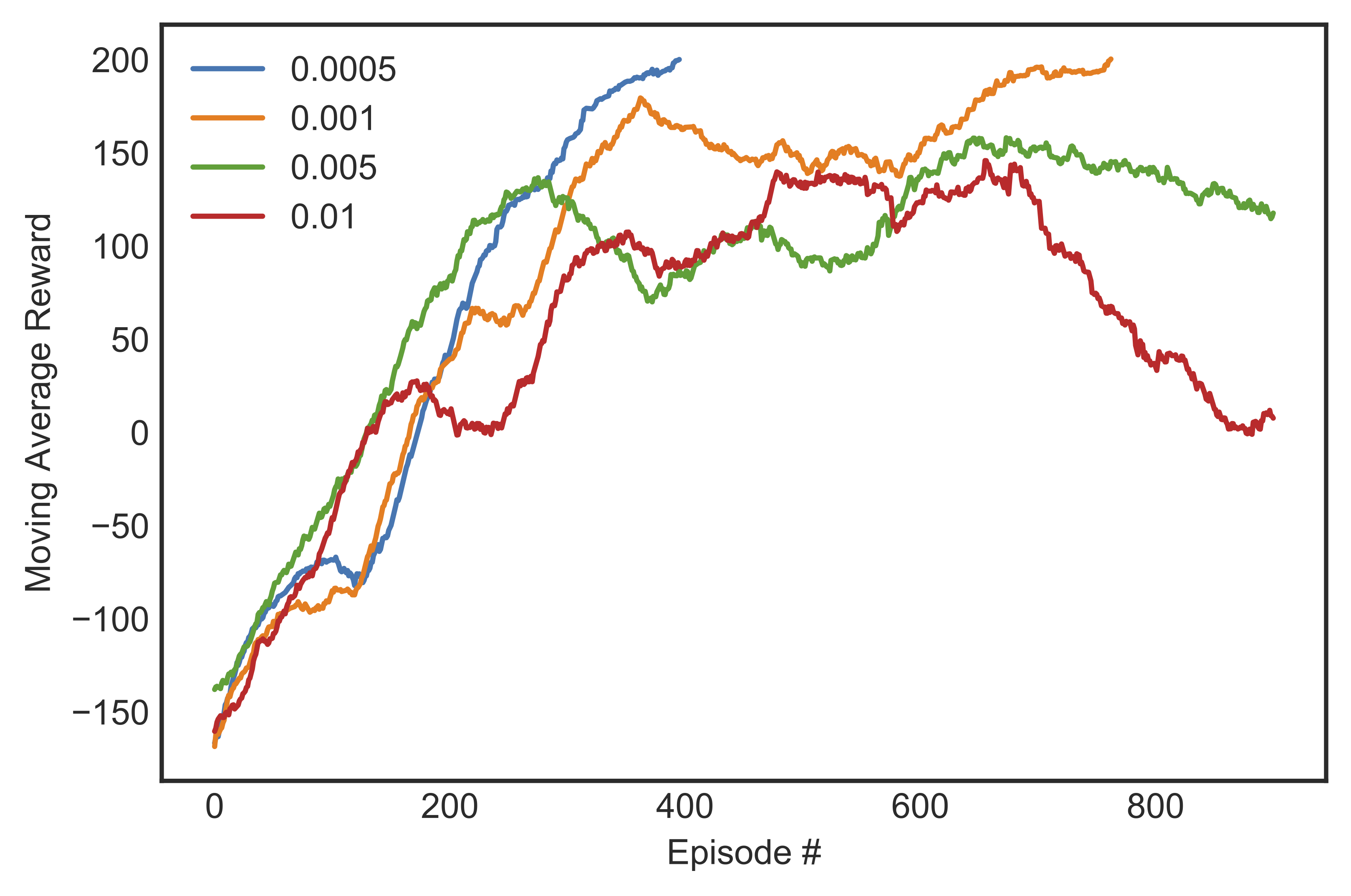{width=”.45textwidth”}

• $alpha=0.01$: The agent almost learned how to land safely, but was too eager to do so. The main engine were turned off sooner than it should have been, resulting in a body-first contact with the ground.

• $alpha=0.005$: The agent was better at landing, although it exhibited different behaviors with different discount rates used. When $gamma=0.99$, more than half of the time the vehicle did not manage to touch the ground within the stipulated time. The rest of the time the vehicle either landed with great accuracy, or cartwheeled to the vast space when it was about to land. When $gamma=0.999$, it didn’t cartwheel, but was too concerned with landing at the right spot that it fired left and right even after it has landed to adjust its horizontal position. Sometimes this strategy backfired and the vehicle fell down the slope and could not crawl back up.

• $alpha=0.001$: The agent completed learning and could consistently land safely most of the time, though when $gamma=0.99$ it still on a few occasions descended a little too fast and landed body-first instead.

• $alpha=0.0005$: When $gamma=0.999$, the agent’s strategy was to descend to a comfortable height, then with the main engine on, slowly hover to a position above the landing pad area by adjusting the left and right engines before finally landing. When $gamma=0.99$, there was no hovering, and hence no horizontal adjustment after descending.

$epsilon$-decay

: Given the complex, continuous state space and the fact that reward only materializes at terminal states, ensuring that the agent adequately explored all state-action combination was important. This is controlled mainly by the $epsilon$ decay rate, which we chose from 0.9, 0.95, 0.99, 0.995, or 0.999. Figure [fig:marewardeps] shows the learning curves for different decay rates with $alpha = 0.001$ and $gamma = 0.999$.

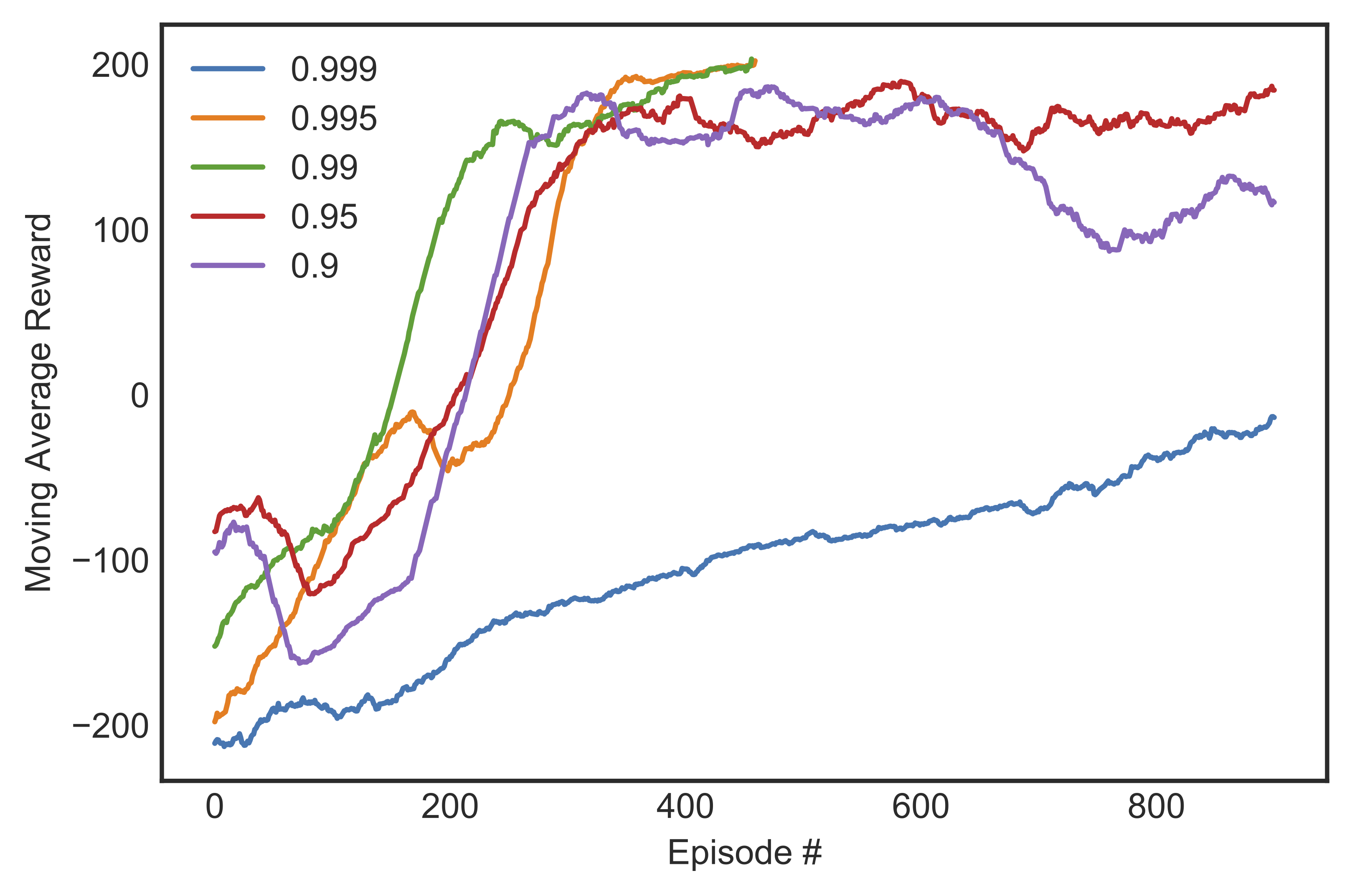{width=”.45textwidth”}

We saw that if the decay rate was too large (0.999) then the agent took too long to learn because it spent all the time exploring new states. If the decay rate was too small (0.9) then the agent started to unlearn after 600 steps or so. A decay rate between 0.99 and 0.995 gave the best result, although the former produced a more stable learning curve.

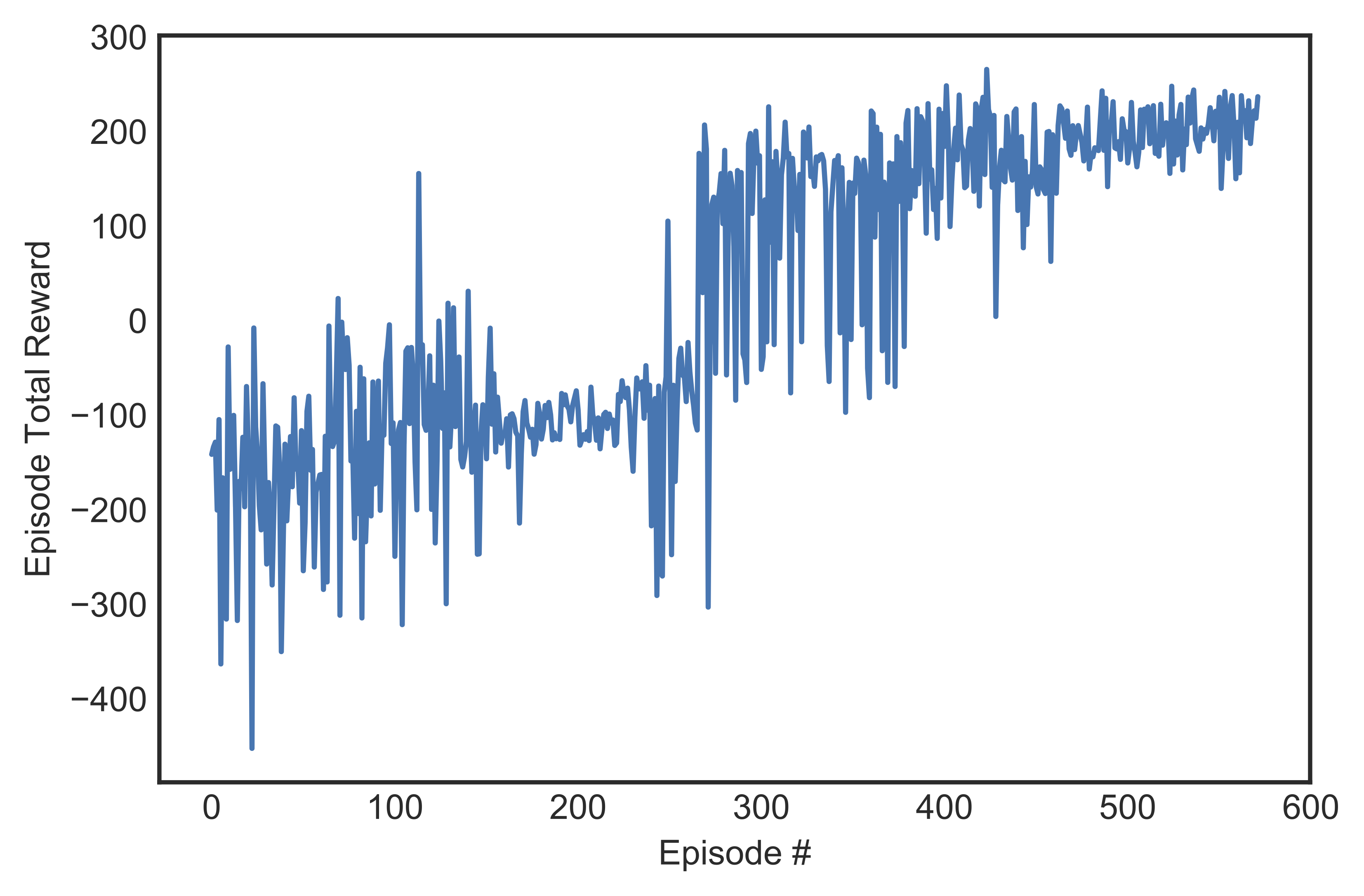
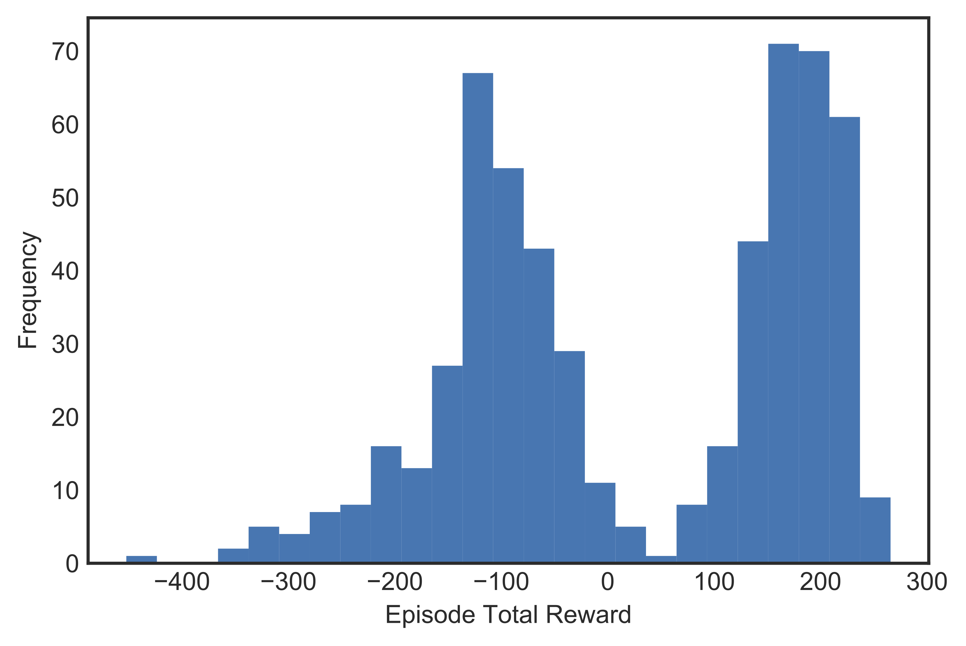
After hyper-parameter tuning, we concluded that the best performing agent was the one that was trained with $alpha = 0.0005$, $gamma = 0.999$, and $epsilon$-decay $= 0.99$. Figure [fig:mabest] shows the learning curve of said agent, which achieved best 100-episode average score of 200.11 within 572 episodes. Figure shows a histogram of total reward earned for each episode while it was learning. The two peaks represent two major learning milestones: the leftmost one was when the lander managed to hover and the rightmost one when it learned to land on target.

{width=”.45textwidth”}

{width=”.45textwidth”}

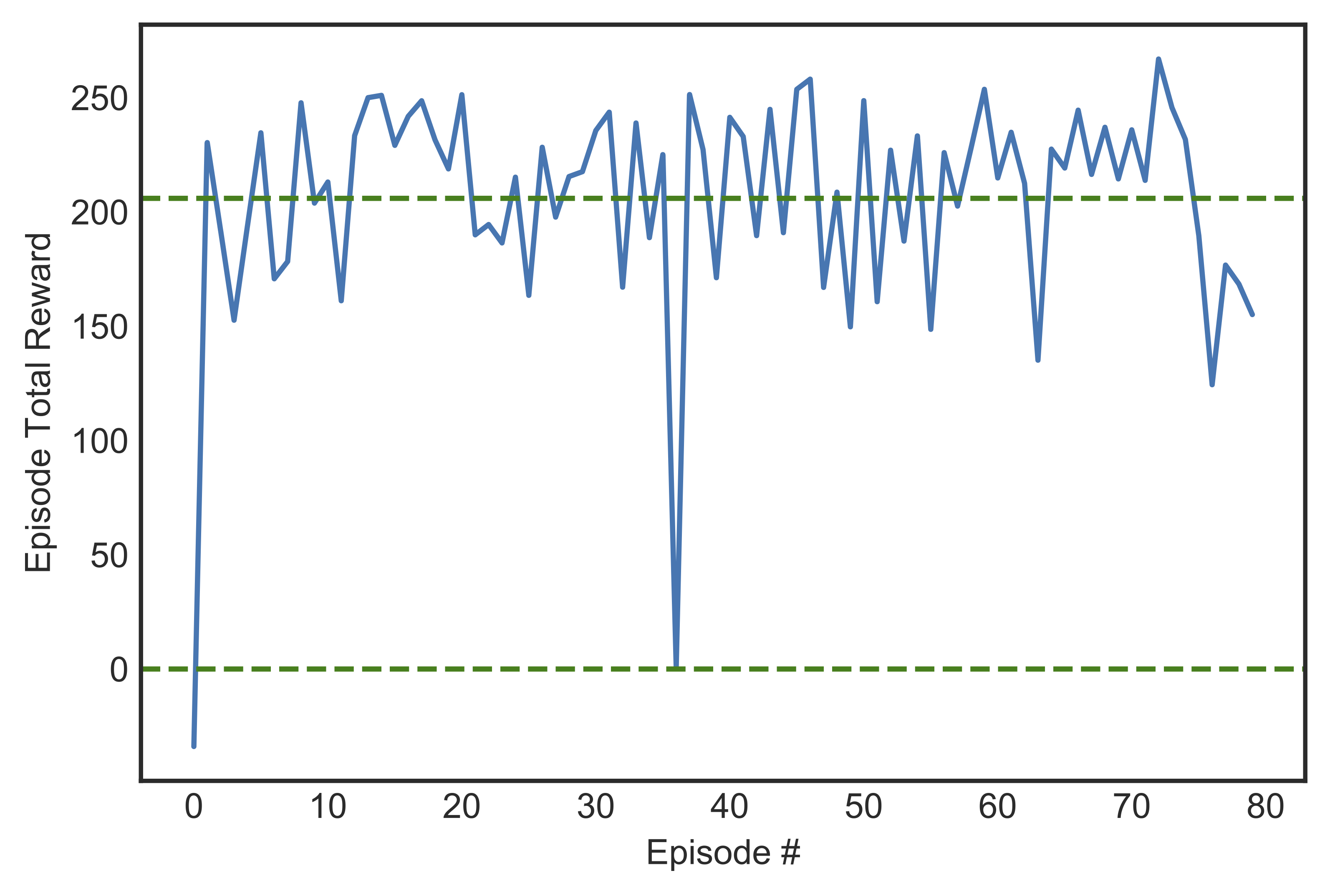
We then let our trained agent run for 100 consecutive episodes without learning and measured its total rewards in Figure [fig:mabesttest]. Only 2 crashes were recorded, and most episodes ended with the vehicle landing safely on the ground (reward more than 100).

{width=”.45textwidth”}

Problems Encountered and Pitfalls

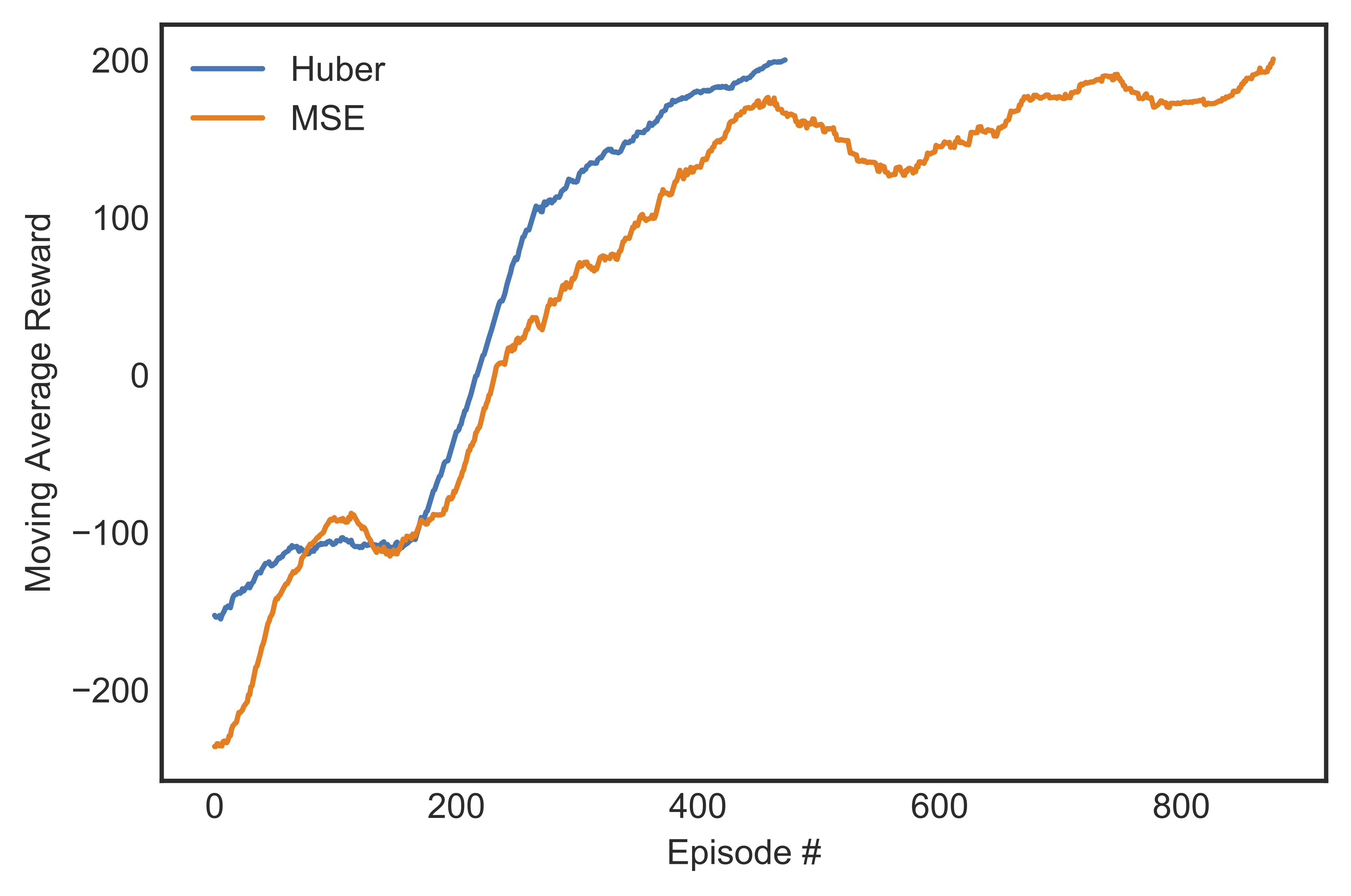
In earlier experiments, we built a network of two fully-connected layers of 64 units each and an output layer, but the learning plateaued from the 500-600th step, at which point the maximum average reward was 130. When we let it continue learning for a few more hundred steps, the score quickly dropped to zero and never recovered to the previous record high. The introduction of an additional 32-unit hidden layer immediately preceding the output layer solved this issue We also experimented with MSE loss before deciding on Huber loss, seeing that the latter could tremendously shorten the training time by 20-30%. Figure [fig:mabesthuber] shows the speed and stability gains from using Huber loss function.

{width=”.45textwidth”}